Where is my direction pole?
Somewhere in a village in Tuscany a direction pole has been installed, and while I was looking around I've asked myself how precise are the distances, and also if giving a glance to the direction pole from one side is possible to triangulate the location.
This is essentially a small exercise of spherical geometry for which Python is perfect. First a look at two photos of the direction pole: it has a total of 18 directions of which 8 pairs of cities share the same direction on opposite faces of the arrow, as shown in the following photos:
 |
| Photo 1 - Cities in Bold |
 |
| Photo 2 |
Continue reading with the details and solution. If you like guessing a place from a picture you can try GeoGuessr that uses Google Street View for creating geographical quizzes.
For the position of the pole we have the coordinates of the village (42.7667 N, 11.7000 E), the coordinates of the pole located using Google Maps (42.775842 N, 11.695500 E) and the one from the phone GPS (42.0160 N, 11.001 E). The location from the phone is not usable differing 100km from the other two. The pole is located about 1km away from the village center.
A map of the locations and the results of the localization can be found on Google Maps (link) thanks to the generated KML file (link).
Then, for every visible city we picked the coordinates using Google and then computed the geodesic distance from the pole location to the city. The errors range from 150m to 80km (12km average), with the bad cases of London (80km) and Buenos Aires (36km). Apart the case of London the relative distance error is between 0.1% and 0.5% of the effective distance. The following plot shows the distribution of errors depending on the distance:
The geodesic distance can be computed with the Vincenty's formula that allows to solve direct and indirect distance problems over the Earh surface.
The next step is the localization based on these distances, and understand if one of the photos is sufficient. One way to perform such a localization is the trilateration that as the name states requires the distances from three points. Over the Earth surface we are interested in the intersection of the geodesic circles centered in each city with given radius. The solution is obtained by expressing each circle as a sphere and intersecting it with the Earth surface. In practice the result is the intersection of four spheres.
Trilateration can be applied to all the 455 triples from the 15 cities and the finding a way to find the best solution. The best triplet taken alone is (Varsavia, Skopje, Vienna) with 19.3 of errors between the estimated location and the real one, while 200 trilaterations failed to be computed. A better result could be obtained by taking the average point among the 455 solutions. But how we can compute the average point from a set of points over the Earth, or at least over a sphere?
A naive approach is the estimation of the center of gravity of the points projected over the sphere, but this results in a point that is 500km away from the real position. A better result can be obtained by finding the point that has the minimum geodesic distance to all the points: equivalently this is a circle fitting over the Earth surface. Non-linear constrained optimization can be used for such an estimation working in 3D and reprojecting the solution over the sphere, or directly working in 2D in the geographical coordinates but using the geodesical distance.
When using the 2D non-linear optimization the resulting "average" trilateration point is not good being 500km from the target.
The non-linear optimization approach can be used for performing multilateration, that is using all the distances at the same time. The objective function to be minimized is the sum of square errors, for each city, of the geodesic distance to the city and the distance reported on the pole. Without using the distance reported on the pole the solution is not unique.
The cities from the two photos get different results, 10km the first set, 42km the second, and then combined 21km. If we remove London from the second set is 10km and the two sets combined gets 7km. For automatically discarding outliers such as London, a RANSAC approach could be employed.
Finally, as a confirmation, the use of the real distances instead of the ones reported on the pole gives an error of the order of 1E-7 km.
The overview of the distances is the following:
Python code for this post can be found on github, using scipy for the non-linear optimization, some elements from the geopy package and pyKML for generating the KML file.
Update: For automating the process the city names and distances could be extracted by means of OCR but this is not an easy task for regular OCR systems, and it also protected by the patent US7917286 "Database assisted OCR for street scenes and other images".
The list of cities with distances in Km are the following, top down, with some missing:
- Unknown
- Unknown - London (1399)
- Berlin (unknown) - Copenhagen (1440)
- Buenos Aires (11175) - San Paolo (9499)
- Varsavia (1262) - Vienna (706)
- Minsk (1700) - Marrakech (2135)
- Kiev (1667) - Mosca (2350)
- Bucarest (1174) - Chisenau (1400)
- Skopje (805) - Sofia (951)
- New York (6794)
For the position of the pole we have the coordinates of the village (42.7667 N, 11.7000 E), the coordinates of the pole located using Google Maps (42.775842 N, 11.695500 E) and the one from the phone GPS (42.0160 N, 11.001 E). The location from the phone is not usable differing 100km from the other two. The pole is located about 1km away from the village center.
A map of the locations and the results of the localization can be found on Google Maps (link) thanks to the generated KML file (link).
 |
| Zoom of the relevant points in Google Earth |
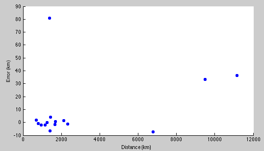 |
| Error of the reported distance against the effective distance |
The geodesic distance can be computed with the Vincenty's formula that allows to solve direct and indirect distance problems over the Earh surface.
The next step is the localization based on these distances, and understand if one of the photos is sufficient. One way to perform such a localization is the trilateration that as the name states requires the distances from three points. Over the Earth surface we are interested in the intersection of the geodesic circles centered in each city with given radius. The solution is obtained by expressing each circle as a sphere and intersecting it with the Earth surface. In practice the result is the intersection of four spheres.
Trilateration can be applied to all the 455 triples from the 15 cities and the finding a way to find the best solution. The best triplet taken alone is (Varsavia, Skopje, Vienna) with 19.3 of errors between the estimated location and the real one, while 200 trilaterations failed to be computed. A better result could be obtained by taking the average point among the 455 solutions. But how we can compute the average point from a set of points over the Earth, or at least over a sphere?
A naive approach is the estimation of the center of gravity of the points projected over the sphere, but this results in a point that is 500km away from the real position. A better result can be obtained by finding the point that has the minimum geodesic distance to all the points: equivalently this is a circle fitting over the Earth surface. Non-linear constrained optimization can be used for such an estimation working in 3D and reprojecting the solution over the sphere, or directly working in 2D in the geographical coordinates but using the geodesical distance.
When using the 2D non-linear optimization the resulting "average" trilateration point is not good being 500km from the target.
The non-linear optimization approach can be used for performing multilateration, that is using all the distances at the same time. The objective function to be minimized is the sum of square errors, for each city, of the geodesic distance to the city and the distance reported on the pole. Without using the distance reported on the pole the solution is not unique.
The cities from the two photos get different results, 10km the first set, 42km the second, and then combined 21km. If we remove London from the second set is 10km and the two sets combined gets 7km. For automatically discarding outliers such as London, a RANSAC approach could be employed.
Finally, as a confirmation, the use of the real distances instead of the ones reported on the pole gives an error of the order of 1E-7 km.
The overview of the distances is the following:
- Minimum distance from trilateration: 19.36km
- Center of Gravity of trilateration points: 500km
- Average location of trilateration points: 504km
- Multilateration without pole distances: 1100km
- Multilateration with pole distance: 21km (7km without London)
- Multilateration with real distances: few cm
 |
| All the points as shown on Google Maps |
Update: For automating the process the city names and distances could be extracted by means of OCR but this is not an easy task for regular OCR systems, and it also protected by the patent US7917286 "Database assisted OCR for street scenes and other images".
Comments